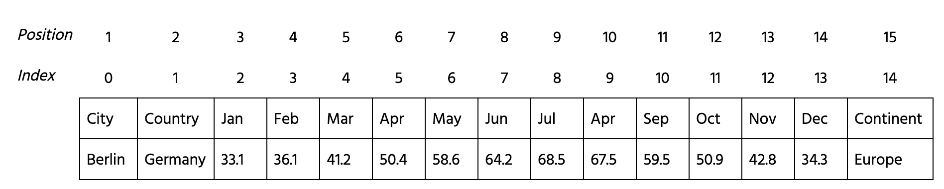
Weather Data: Complete and Ward Linkages

The last chart was good, but if you remember the K-Means and K-Medoids algorithms results, you may remember that there was at least one more line that unlike all the others goes downwards close to July. The average linkage in hierarchical clustering didn't catch that dynamic.

We saw that for complete and ward linkages there is sense to consider 4 clusters. Let's find out will they catch that?

Tâche

Swipe to start coding

Import numpy with np alias.
Iterate over the linkages list. At each step:

Create a hierarchical clustering model with 4 clusters and method j named model.
Fit the numerical data of temp and predict the labels. Add predicted labels as the 'prediction' column to temp.
Create a temp_res DataFrame with monthly averages for each group. To do it group the values of temp by the 'prediction' column, calculate the mean, and then apply the .stack() method.
Add column 'method' to temp_res DataFrame with value j being repeated the number of rows in temp_res times.
Merge res and temp_res dataframes using .concat function of pd.

Reassign the column names of res to ['Group', 'Month', 'Temp', "Method"].
Within the FacetGrid function set the col parameter to 'Method'. This will build a separate chart for each value of the 'Method' column.
Within the .map function set the seaborn line plot function as the first parameter.

Solution

# Import the librarires

import pandas as pd

import seaborn as sns

import matplotlib.pyplot as plt

from sklearn.cluster import AgglomerativeClustering

import numpy as np

# Read the data

data = pd.read_csv('https://codefinity-content-media.s3.eu-west-1.amazonaws.com/138ab9ad-aa37-4310-873f-0f62abafb038/Cities+weather.csv', index_col = 0)

# Empty DataFrame and list of methods

res = pd.DataFrame()

linkages = ['complete', 'ward']

# Iterate over methods

for j in linkages:

temp = data

# Create the model

model = AgglomerativeClustering(n_clusters = 4, linkage = j)

# Fit the data and predict the labels

temp['prediction'] = model.fit_predict(temp.iloc[:,2:14])

col = list(data.columns[2:14]) + ['prediction']

# Calculate mean across each month and group

temp_res = temp[col].groupby('prediction').mean().stack().reset_index()

# Add column with method's name

temp_res['method'] = np.repeat(j, len(temp_res))

# Add resulted DataFrame to res

res = pd.concat([res, temp_res])

# Assign new column names

res.columns = ['Group', 'Month', "Temp", "Method"]

# Visualize the results

g = sns.FacetGrid(res, col = 'Method')

g.map(sns.lineplot, "Month", "Temp", "Group")

plt.show()

Tout était clair ?

Merci pour vos commentaires !

Section 3. Chapitre 7

# Import the librarires

import pandas as pd

import seaborn as sns

import matplotlib.pyplot as plt

from sklearn.cluster import AgglomerativeClustering

import ___

# Read the data

data = pd.read_csv('https://codefinity-content-media.s3.eu-west-1.amazonaws.com/138ab9ad-aa37-4310-873f-0f62abafb038/Cities+weather.csv', index_col = 0)

# Empty DataFrame and list of methods

res = pd.DataFrame()

linkages = ['complete', 'ward']

# Iterate over methods

for j in linkages:

temp = data

# Create the model

model = ___(___ = ___, linkage = ___)

# Fit the data and predict the labels

temp['prediction'] = model.___(___.___[:,2:14])

col = list(data.columns[2:14]) + ['prediction']

# Calculate mean across each month and group

temp_res = temp[col].groupby('___').___().___().reset_index()

# Add column with method's name

temp_res['method'] = np.repeat(j, ___)

# Add resulted DataFrame to res

res = pd.___([res, ___])

# Assign new column names

res.___ = ['Group', 'Month', 'Temp', 'Method']

# Visualize the results

g = sns.FacetGrid(res, col = '___')

g.map(___, "Month", "Temp", "Group")

plt.show()

Demandez à l'IA

Posez n'importe quelle question ou essayez l'une des questions suggérées pour commencer notre discussion