Creating PivotTables with VBA
Swipe to show menu
A PivotTable summarizes a table by dragging fields into Rows, Columns, and Values — and every one of those drag-and-drop actions has a direct VBA equivalent, which means an entire PivotTable report can be rebuilt from scratch by a macro every time new data arrives.
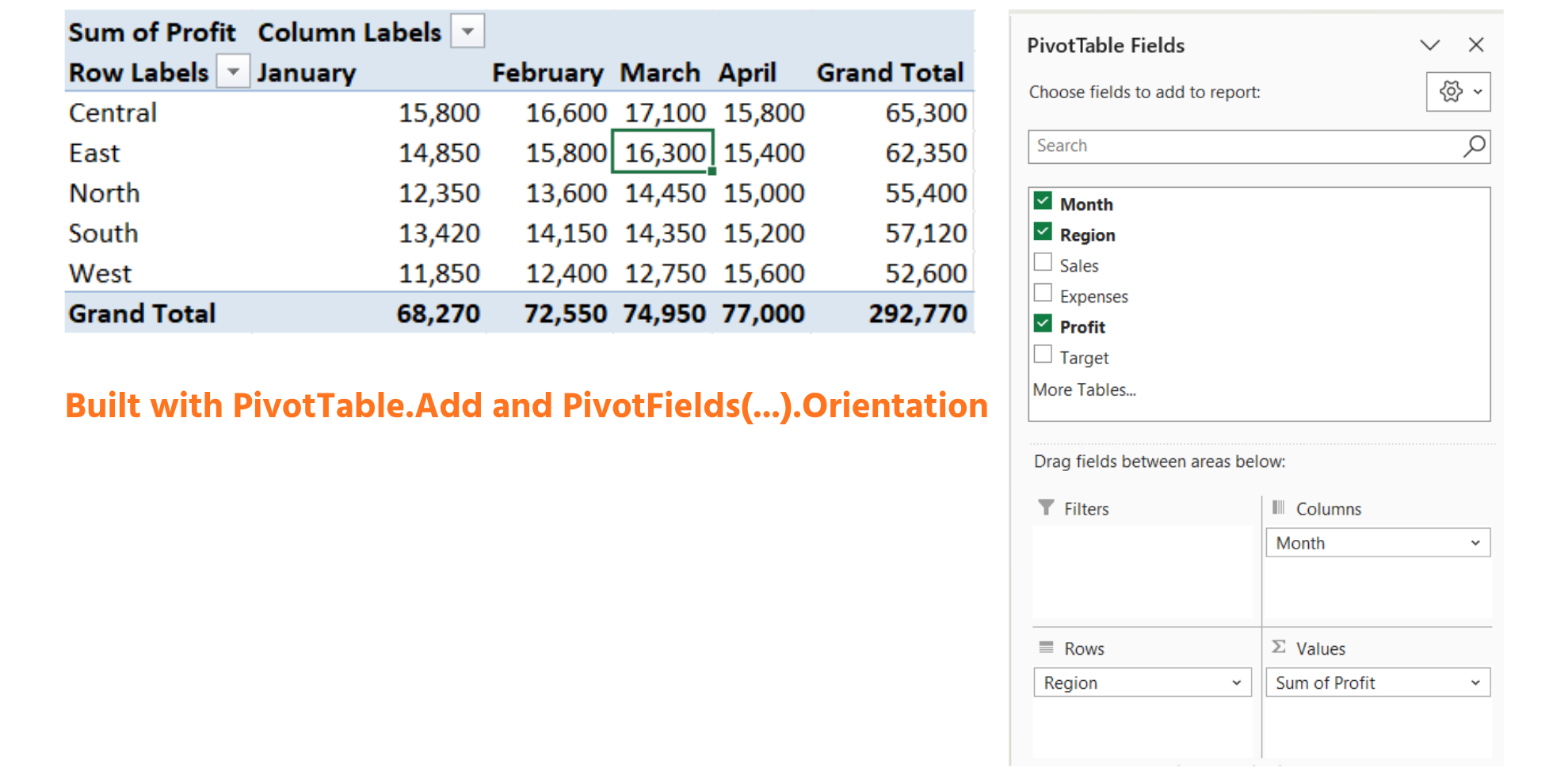
Building a PivotTable
Sub BuildProfitPivot()
    Dim wsData As Worksheet, wsPivot As Worksheet
    Dim tbl As ListObject
    Dim pc As PivotCache
    Dim pt As PivotTable

    Set wsData = ThisWorkbook.Worksheets("Reports")
    Set tbl = wsData.ListObjects("tblReports")

    ' start clean: remove an existing Pivot sheet if this has run before
    On Error Resume Next
    Application.DisplayAlerts = False
    ThisWorkbook.Worksheets("Pivot").Delete
    Application.DisplayAlerts = True
    On Error GoTo 0

    Set wsPivot = ThisWorkbook.Worksheets.Add
    wsPivot.Name = "Pivot"

    Set pc = ThisWorkbook.PivotCaches.Create( _
        SourceType:=xlDatabase, SourceData:=tbl.Range)

    Set pt = pc.CreatePivotTable( _
        TableDestination:=wsPivot.Range("A3"), _
        TableName:="ptProfitByRegion")

    With pt
        .PivotFields("Region").Orientation = xlRowField
        .PivotFields("Month").Orientation = xlColumnField
        .AddDataField .PivotFields("Profit"), "Sum of Profit", xlSum
    End With
End Sub

- On Error Resume Next paired with the
DisplayAlertstoggle and.Deleteis a safe "delete if it exists" pattern: deleting a sheet that doesn't exist would normally throw an error and stop the macro, but On Error Resume Next tells VBA to quietly continue past that specific error instead;DisplayAlerts = Falsesuppresses Excel's own "are you sure you want to delete this sheet?" confirmation popup; - On
Error GoTo 0immediately afterward turns normal error-reporting back on — leavingOn Error Resume Nextactive for the rest of theSubwould silently swallow any later, unrelated errors too, which is a trap worth avoiding; ThisWorkbook.PivotCaches.Createtakes a snapshot of the Table's data — the PivotCache, not the PivotTable itself — which is the object every PivotTable is actually built from behind the scenes;pc.CreatePivotTableis what turns that snapshot into a visible PivotTable, placed starting at cell A3 on the new Pivot sheet and given the name ptProfitByRegion so later code (RefreshTable, for instance) can find it again by name;PivotFields("Region").Orientation = xlRowFieldand the Month line immediately below it are the direct code equivalent of dragging Region into the Rows box and Month into the Columns box in the Field List;AddDataFieldis what populates the Values area — the second argument ("Sum of Profit") is just the label Excel displays as the column heading, and xlSum tells it to add the values rather than average or count them.
Refreshing Reports
Once a PivotTable exists, you don't rebuild it every time new data arrives — you refresh it, which is faster and preserves any manual layout tweaks a user made:
ThisWorkbook.Worksheets("Pivot").PivotTables("ptProfitByRegion").RefreshTable
This single line re-reads the PivotCache from the current state of tblReports and updates every number in the PivotTable to match — but it leaves the layout exactly as it is, including any column widths, number formatting, or field arrangement a user adjusted by hand after the Pivot was first built. That's the key advantage over calling BuildProfitPivot again: rebuilding from scratch would recreate the sheet and wipe out any of those manual tweaks.
Updating PivotCharts
A PivotChart built on top of a PivotTable updates its data automatically whenever the PivotTable refreshes — so refreshing the table is usually all a report macro needs to do to keep an attached chart current too:
Dim pt As PivotTable
Set pt = ThisWorkbook.Worksheets("Pivot").PivotTables("ptProfitByRegion")
pt.RefreshTable
' any PivotChart based on pt updates automatically — no extra code needed
This is worth contrasting with the ordinary charts covered in the next section: a regular chart needs an explicit SetSourceData call to point it at new data, while a PivotChart is permanently linked to its PivotTable and simply follows along for free. If a dashboard needs a chart that always reflects the latest PivotTable numbers with the least code, building it as a PivotChart rather than a standalone chart is usually the better choice.
Task
- Run
BuildProfitPivotexactly as shown and confirm a new "Pivot" sheet appears with Region down the rows and Month across the columns. - Manually add a new March row to
tblReportsfor a fictional sixth region, then run only the RefreshTable line — confirm the Pivot updates without rebuilding it from scratch. - Modify
BuildProfitPivotto summarize Sales instead of Profit, and swap Region and Month so Month is in Rows and Region is in Columns.
Here's the code to add a sixth region as a new March row in tblReports, using ListRows.Add instead of typing it in manually:
Sub AddSixthRegion()
    Dim tbl As ListObject
    Dim newRow As ListRow

    Set tbl = ThisWorkbook.Worksheets("Reports").ListObjects("tblReports")
    Set newRow = tbl.ListRows.Add

    newRow.Range(1, 1).Value = "March"        ' Month
    newRow.Range(1, 2).Value = "Southwest"    ' Region
    newRow.Range(1, 3).Value = 41500          ' Sales
    newRow.Range(1, 4).Value = 28200          ' Expenses
    newRow.Range(1, 5).Value = 13300          ' Profit
    newRow.Range(1, 6).Value = 39000          ' Target
End Sub
Run this once, then run the RefreshProfitPivot Sub from before — the Pivot table should now show "Southwest" as a new row alongside North, South, East, West, and Central, without you having touched the Pivot-building macro at all.
1. Running BuildProfitPivot as-is
- Copy the
Subexactly as written in chapter into your module and run it once. - Check the Project Explorer or your sheet tabs — a new sheet literally named "Pivot" should appear, with Region listed down the rows and Month spread across the columns, summing Profit.
2. Adding a sixth region and refreshing only
- Type the new row directly into the worksheet (not through code) — go to the bottom of
tblReportsand add a March row for a made-up region, e.g. "Southwest." - Don't re-run
BuildProfitPivot— that would delete and rebuild the whole Pivot sheet from scratch, which defeats the point of this exercise. - Instead, run only the one-line
RefreshTablestatement from chapter — you'll need to reference the existing PivotTable by name, the same way the chapter's own refresh example did.
3. Swapping fields and changing the summarized value
- Three lines inside the
With ptblock need to change: which field isxlRowField, which isxlColumnField, and which fieldAddDataFieldpoints at. - Give this modified version a different
Subname and a differentTableName— reusing the same names as the original would either error or silently overwrite the first Pivot table. - The label passed to
AddDataField(the second argument, like"Sum of Profit") is just display text — update it to match whatever you're actually summarizing now.
Point 2 — after manually adding the sixth region's row, run just this:
Sub RefreshProfitPivot()
    ThisWorkbook.Worksheets("Pivot").PivotTables("ptProfitByRegion").RefreshTable
End Sub
Point 3 — a separate, modified version:
Sub BuildSalesPivotByMonth()
    Dim wsData As Worksheet, wsPivot As Worksheet
    Dim tbl As ListObject
    Dim pc As PivotCache
    Dim pt As PivotTable

    Set wsData = ThisWorkbook.Worksheets("Reports")
    Set tbl = wsData.ListObjects("tblReports")

    On Error Resume Next
    Application.DisplayAlerts = False
    ThisWorkbook.Worksheets("SalesPivot").Delete
    Application.DisplayAlerts = True
    On Error GoTo 0

    Set wsPivot = ThisWorkbook.Worksheets.Add
    wsPivot.Name = "SalesPivot"

    Set pc = ThisWorkbook.PivotCaches.Create( _
        SourceType:=xlDatabase, SourceData:=tbl.Range)

    Set pt = pc.CreatePivotTable( _
        TableDestination:=wsPivot.Range("A3"), _
        TableName:="ptSalesByMonth")

    With pt
        .PivotFields("Month").Orientation = xlRowField
        .PivotFields("Region").Orientation = xlColumnField
        .AddDataField .PivotFields("Sales"), "Sum of Sales", xlSum
    End With
End Sub
Run BuildSalesPivotByMonth and you should get a new "SalesPivot" sheet with Month down the rows, Region across the columns, and Sales totals in the body — the mirror image of the original layout.
Thanks for your feedback!
Ask AI

Ask AI

Ask anything or try one of the suggested questions to begin our chat
