Notice: This page requires JavaScript to function properly.
Please enable JavaScript in your browser settings or update your browser.
Learn Model Training | Neural Network from Scratch
Introduction to Neural Networks with Python

Model Training

Swipe to show menu

Training a neural network involves an iterative process in which the model gradually improves by adjusting its weights and biases to minimize the loss function. This process is known as gradient-based optimization, and it follows a structured algorithm.

General Algorithm

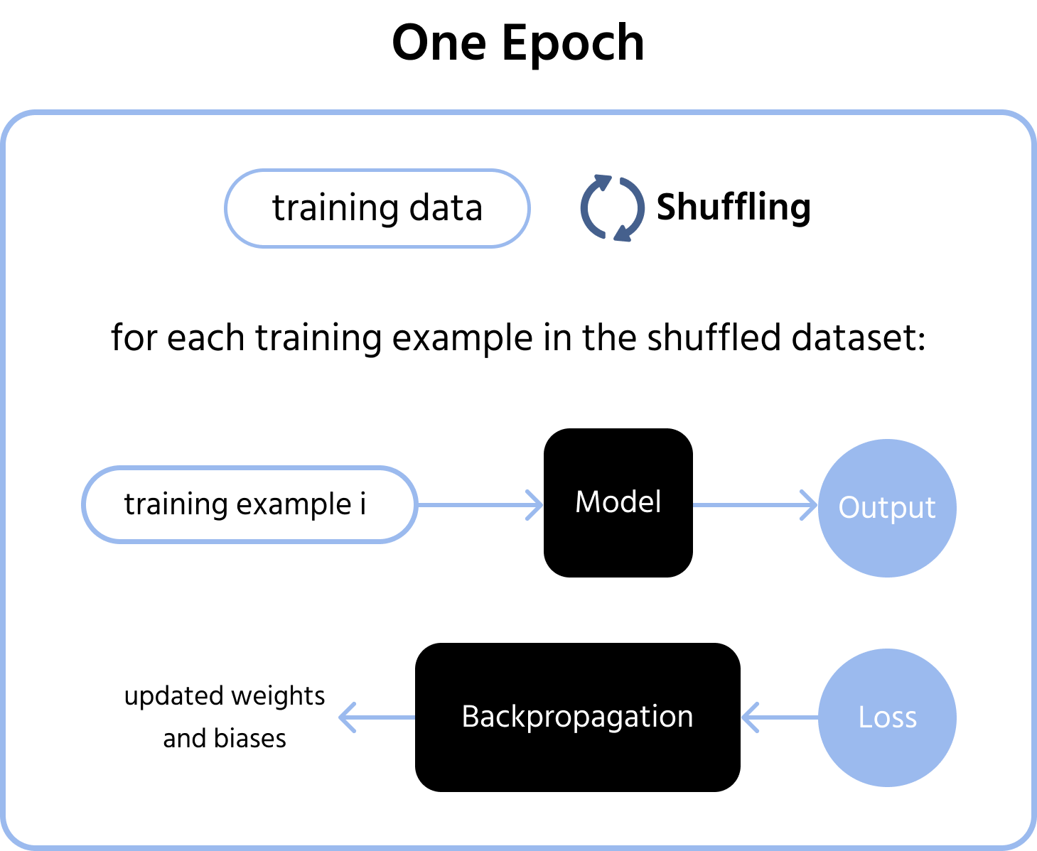
The dataset is first passed through the network multiple times in a loop, where each complete pass is referred to as an epoch. During each epoch, the data is shuffled to prevent the model from learning patterns based on the order of the training examples. Shuffling helps introduce randomness, leading to a more robust model.

For each training example, the model performs forward propagation, where inputs pass through the network, layer by layer, producing an output. This output is then compared to the actual target value to compute the loss.
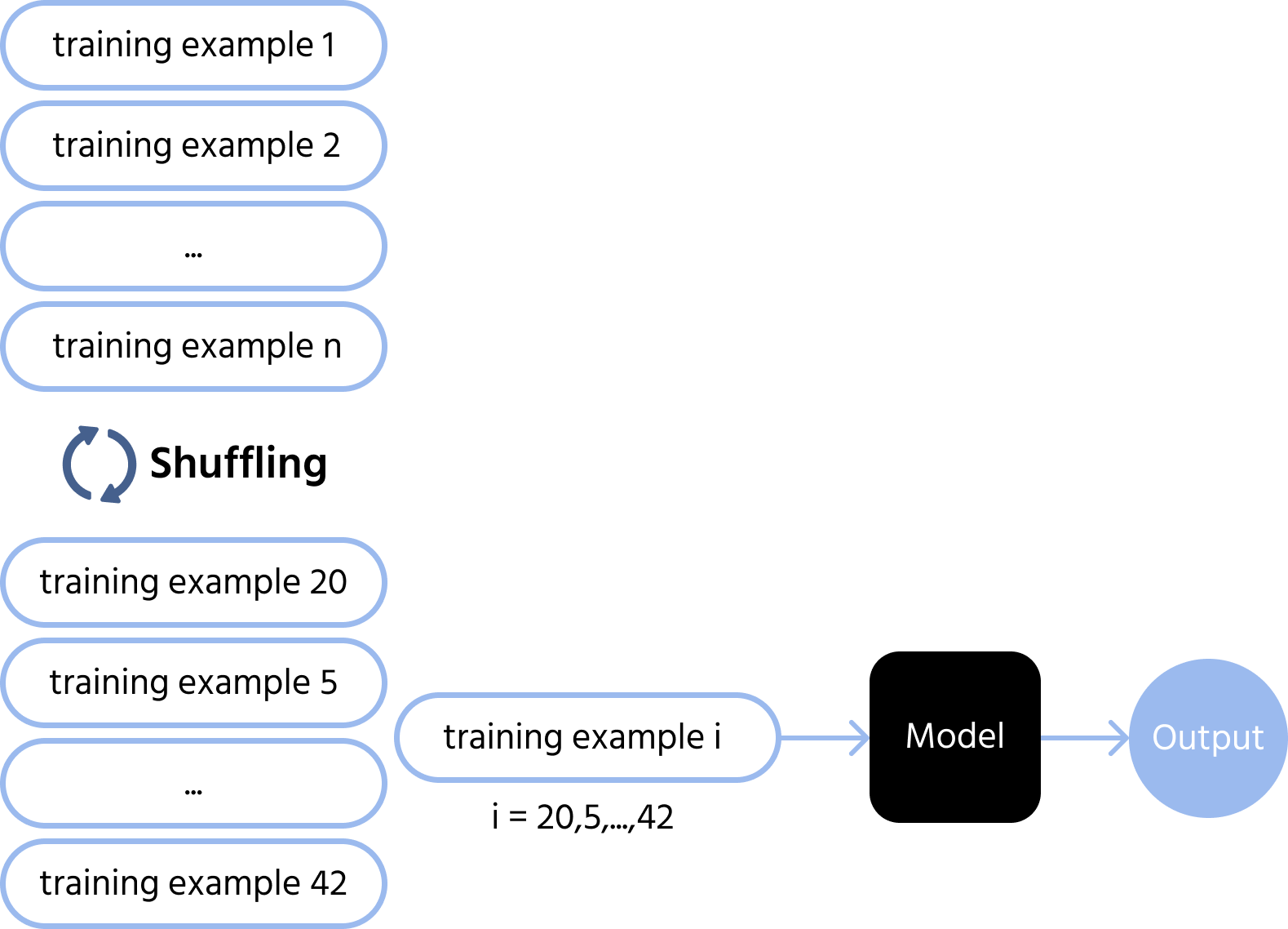
Shuffling and forward propagation

Next, the model applies backpropagation and updates the weights and biases in each layer to reduces the loss.

This process repeats for multiple epochs, allowing the network to refine its parameters gradually. As training progresses, the network learns to make increasingly accurate predictions. However, careful tuning of hyperparameters such as the learning rate is crucial to ensure stable and efficient training.
Epoch

The learning rate (α\alpha) determines the step size in weight updates. If it is too high, the model might overshoot the optimal values and fail to converge. If it is too low, training becomes slow and might get stuck in a suboptimal solution. Choosing an appropriate learning rate balances speed and stability in training. Typical values range from 0.001 to 0.1, depending on the problem and network size.

The graph below shows how an appropriate learning rate enables the loss to decrease steadily at an optimal pace:
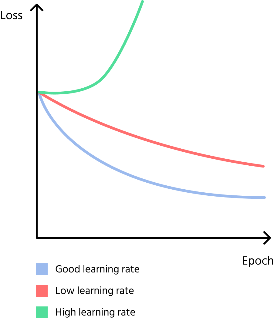
Different learning rates

Finally, stochastic gradient descent (SGD) plays a vital role in training efficiency. Instead of computing weight updates after processing the entire dataset, SGD updates the parameters after each individual example. This makes training faster and introduces slight variations in updates, which can help the model escape local minima and reach a better overall solution.

The fit() Method

The fit() method in the Perceptron class is responsible for training the model using stochastic gradient descent.

def fit(self, training_data, labels, epochs, learning_rate):
    # Iterating over multiple epochs
    for epoch in range(epochs):
        # Shuffling the data  
        indices = np.random.permutation(training_data.shape[0])
        training_data = training_data[indices]
        labels = labels[indices]
        # Iterating through each training example
        for i in range(training_data.shape[0]):
            inputs = training_data[i, :].reshape(-1, 1)
            target = labels[i, :].reshape(-1, 1)

            # Forward propagation
            output = ...

            # Computing the gradient of the loss function w.r.t. output
            da = ...

            # Backward propagation through all layers
            for layer in self.layers[::-1]:
                da = ...
Code Description
expand arrow
for epoch in range(epochs):

Loops through the training process for the given number of epochs. Each epoch represents one full pass over the dataset.

indices = np.random.permutation(training_data.shape[0])
training_data = training_data[indices]
labels = labels[indices]

Shuffles the training data and corresponding labels before each epoch. This prevents the model from learning patterns based on data order.

for i in range(training_data.shape[0]):

Iterates through each training examples. Since SGD is used, weights are updated after processing each individual example.

inputs = training_data[i, :].reshape(-1, 1)
target = labels[i, :].reshape(-1, 1)

Extracts the i-th training example and its label. Reshapes them into n x 1 matrix for matrix operations to work correctly.

output = ...

Performs forward propagation to compute the predicted output.

da = ...

Computes the gradient of the loss function with respect to the output activation. This serves as the starting gradient for backpropagation.

for layer in self.layers[::-1]:
    da = ...

Performs backward propagation through all layers in reverse order. Each layer updates its weights and biases using gradient descent.

question mark

What is one complete pass through the entire training dataset called?

Select the correct answer

Everything was clear?

How can we improve it?

Thanks for your feedback!

Section 2. Chapter 9

Ask AI

expand

Ask AI

ChatGPT

Ask anything or try one of the suggested questions to begin our chat

Model Training

Training a neural network involves an iterative process in which the model gradually improves by adjusting its weights and biases to minimize the loss function. This process is known as gradient-based optimization, and it follows a structured algorithm.

General Algorithm

The dataset is first passed through the network multiple times in a loop, where each complete pass is referred to as an epoch. During each epoch, the data is shuffled to prevent the model from learning patterns based on the order of the training examples. Shuffling helps introduce randomness, leading to a more robust model.

For each training example, the model performs forward propagation, where inputs pass through the network, layer by layer, producing an output. This output is then compared to the actual target value to compute the loss.

Shuffling and forward propagation

Next, the model applies backpropagation and updates the weights and biases in each layer to reduces the loss.

This process repeats for multiple epochs, allowing the network to refine its parameters gradually. As training progresses, the network learns to make increasingly accurate predictions. However, careful tuning of hyperparameters such as the learning rate is crucial to ensure stable and efficient training.

Epoch

The learning rate (α\alpha) determines the step size in weight updates. If it is too high, the model might overshoot the optimal values and fail to converge. If it is too low, training becomes slow and might get stuck in a suboptimal solution. Choosing an appropriate learning rate balances speed and stability in training. Typical values range from 0.001 to 0.1, depending on the problem and network size.

The graph below shows how an appropriate learning rate enables the loss to decrease steadily at an optimal pace:

Different learning rates

Finally, stochastic gradient descent (SGD) plays a vital role in training efficiency. Instead of computing weight updates after processing the entire dataset, SGD updates the parameters after each individual example. This makes training faster and introduces slight variations in updates, which can help the model escape local minima and reach a better overall solution.

The fit() Method

The fit() method in the Perceptron class is responsible for training the model using stochastic gradient descent.

def fit(self, training_data, labels, epochs, learning_rate):
    # Iterating over multiple epochs
    for epoch in range(epochs):
        # Shuffling the data  
        indices = np.random.permutation(training_data.shape[0])
        training_data = training_data[indices]
        labels = labels[indices]
        # Iterating through each training example
        for i in range(training_data.shape[0]):
            inputs = training_data[i, :].reshape(-1, 1)
            target = labels[i, :].reshape(-1, 1)

            # Forward propagation
            output = ...

            # Computing the gradient of the loss function w.r.t. output
            da = ...

            # Backward propagation through all layers
            for layer in self.layers[::-1]:
                da = ...
Code Description
expand arrow
for epoch in range(epochs):

Loops through the training process for the given number of epochs. Each epoch represents one full pass over the dataset.

indices = np.random.permutation(training_data.shape[0])
training_data = training_data[indices]
labels = labels[indices]

Shuffles the training data and corresponding labels before each epoch. This prevents the model from learning patterns based on data order.

for i in range(training_data.shape[0]):

Iterates through each training examples. Since SGD is used, weights are updated after processing each individual example.

inputs = training_data[i, :].reshape(-1, 1)
target = labels[i, :].reshape(-1, 1)

Extracts the i-th training example and its label. Reshapes them into n x 1 matrix for matrix operations to work correctly.

output = ...

Performs forward propagation to compute the predicted output.

da = ...

Computes the gradient of the loss function with respect to the output activation. This serves as the starting gradient for backpropagation.

for layer in self.layers[::-1]:
    da = ...

Performs backward propagation through all layers in reverse order. Each layer updates its weights and biases using gradient descent.

Everything was clear?

How can we improve it?

Thanks for your feedback!

Section 2. Chapter 9
some-alt