Implementando Word2Vec
Deslize para mostrar o menu
Após compreender como o Word2Vec funciona, prossiga para implementá-lo utilizando Python. A biblioteca Gensim, uma ferramenta robusta e de código aberto para processamento de linguagem natural, oferece uma implementação direta por meio da classe Word2Vec em gensim.models.
Preparação dos Dados
O Word2Vec exige que os dados textuais estejam tokenizados, ou seja, divididos em uma lista de listas, onde cada lista interna contém as palavras de uma sentença específica. Neste exemplo, será utilizado o romance Emma da autora inglesa Jane Austen como corpus. Um arquivo CSV contendo sentenças pré-processadas será carregado e, em seguida, cada sentença será dividida em palavras:
12345678import pandas as pd emma_df = pd.read_csv( 'https://content-media-cdn.codefinity.com/courses/c68c1f2e-2c90-4d5d-8db9-1e97ca89d15e/section_4/chapter_3/emma.csv') # Split each sentence into words sentences = emma_df['Sentence'].str.split() # Print the fourth sentence (list of words) print(sentences[3])
emma_df['Sentence'].str.split() aplica o método .split() a cada sentença na coluna 'Sentence', resultando em uma lista de palavras para cada sentença. Como as sentenças já foram pré-processadas, com as palavras separadas por espaços em branco, o método .split() é suficiente para essa tokenização.
Treinamento do Modelo Word2Vec
Agora, o foco é o treinamento do modelo Word2Vec utilizando os dados tokenizados. A classe Word2Vec oferece uma variedade de parâmetros para personalização. No entanto, os parâmetros mais comuns são:
vector_size(100 por padrão): dimensionalidade ou tamanho dos embeddings de palavras;window(5 por padrão): tamanho da janela de contexto;min_count(5 por padrão): palavras que ocorrem menos vezes que esse valor serão ignoradas;sg(0 por padrão): arquitetura do modelo a ser utilizada (1 para Skip-gram, 0 para CBoW).cbow_mean(1 por padrão): especifica se o contexto de entrada do CBoW é somado (0) ou calculada a média (1)
Sobre as arquiteturas do modelo, CBoW é adequado para conjuntos de dados maiores e cenários onde a eficiência computacional é essencial. Skip-gram, por outro lado, é preferível para tarefas que exigem compreensão detalhada dos contextos das palavras, sendo particularmente eficaz em conjuntos de dados menores ou ao lidar com palavras raras.
12345678from gensim.models import Word2Vec import pandas as pd emma_df = pd.read_csv( 'https://content-media-cdn.codefinity.com/courses/c68c1f2e-2c90-4d5d-8db9-1e97ca89d15e/section_4/chapter_3/emma.csv') sentences = emma_df['Sentence'].str.split() # Initialize the model model = Word2Vec(sentences, vector_size=200, window=5, min_count=1, sg=0)
Aqui, definimos o tamanho do embedding como 200, o tamanho da janela de contexto como 5 e incluímos todas as palavras ao definir min_count=1. Ao definir sg=0, optamos por utilizar o modelo CBoW.
A escolha do tamanho do embedding e da janela de contexto envolve compensações. Embeddings maiores capturam mais significado, mas aumentam o custo computacional e o risco de overfitting. Janelas de contexto menores são mais eficazes para capturar sintaxe, enquanto janelas maiores são melhores para capturar semântica.
Encontrando Palavras Semelhantes
Uma vez que as palavras são representadas como vetores, é possível compará-las para medir similaridade. Embora seja possível utilizar distância, a direção de um vetor frequentemente carrega mais significado semântico do que sua magnitude, especialmente em embeddings de palavras.
No entanto, utilizar o ângulo como métrica de similaridade diretamente não é tão conveniente. Em vez disso, pode-se usar o cosseno do ângulo entre dois vetores, também conhecido como similaridade do cosseno. Ela varia de -1 a 1, com valores mais altos indicando maior similaridade. Essa abordagem foca em quão alinhados os vetores estão, independentemente do comprimento, tornando-a ideal para comparar significados de palavras. Veja uma ilustração:
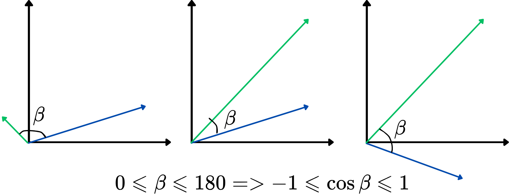
Quanto maior a similaridade do cosseno, mais semelhantes são os dois vetores, e vice-versa. Por exemplo, se dois vetores de palavras possuem uma similaridade do cosseno próxima de 1 (ângulo próximo de 0 graus), isso indica que eles estão intimamente relacionados ou são semelhantes em contexto dentro do espaço vetorial.
Agora, vamos encontrar as 5 palavras mais semelhantes à palavra "man" utilizando a similaridade do cosseno:
12345678910from gensim.models import Word2Vec import pandas as pd emma_df = pd.read_csv( 'https://content-media-cdn.codefinity.com/courses/c68c1f2e-2c90-4d5d-8db9-1e97ca89d15e/section_4/chapter_3/emma.csv') sentences = emma_df['Sentence'].str.split() model = Word2Vec(sentences, vector_size=200, window=5, min_count=1, sg=0) # Retrieve the top-5 most similar words to 'man' similar_words = model.wv.most_similar('man', topn=5) print(similar_words)
model.wv acessa os vetores de palavras do modelo treinado, enquanto o método .most_similar() encontra as palavras cujos embeddings estão mais próximos do embedding da palavra especificada, com base na similaridade do cosseno. O parâmetro topn determina o número de top-N palavras semelhantes a serem retornadas.
Obrigado pelo seu feedback!
Pergunte à IA
Pergunte à IA

Pergunte o que quiser ou experimente uma das perguntas sugeridas para iniciar nosso bate-papo
Implementando Word2Vec
Após compreender como o Word2Vec funciona, prossiga para implementá-lo utilizando Python. A biblioteca Gensim, uma ferramenta robusta e de código aberto para processamento de linguagem natural, oferece uma implementação direta por meio da classe Word2Vec em gensim.models.
Preparação dos Dados
O Word2Vec exige que os dados textuais estejam tokenizados, ou seja, divididos em uma lista de listas, onde cada lista interna contém as palavras de uma sentença específica. Neste exemplo, será utilizado o romance Emma da autora inglesa Jane Austen como corpus. Um arquivo CSV contendo sentenças pré-processadas será carregado e, em seguida, cada sentença será dividida em palavras:
12345678import pandas as pd emma_df = pd.read_csv( 'https://content-media-cdn.codefinity.com/courses/c68c1f2e-2c90-4d5d-8db9-1e97ca89d15e/section_4/chapter_3/emma.csv') # Split each sentence into words sentences = emma_df['Sentence'].str.split() # Print the fourth sentence (list of words) print(sentences[3])
emma_df['Sentence'].str.split() aplica o método .split() a cada sentença na coluna 'Sentence', resultando em uma lista de palavras para cada sentença. Como as sentenças já foram pré-processadas, com as palavras separadas por espaços em branco, o método .split() é suficiente para essa tokenização.
Treinamento do Modelo Word2Vec
Agora, o foco é o treinamento do modelo Word2Vec utilizando os dados tokenizados. A classe Word2Vec oferece uma variedade de parâmetros para personalização. No entanto, os parâmetros mais comuns são:
vector_size(100 por padrão): dimensionalidade ou tamanho dos embeddings de palavras;window(5 por padrão): tamanho da janela de contexto;min_count(5 por padrão): palavras que ocorrem menos vezes que esse valor serão ignoradas;sg(0 por padrão): arquitetura do modelo a ser utilizada (1 para Skip-gram, 0 para CBoW).cbow_mean(1 por padrão): especifica se o contexto de entrada do CBoW é somado (0) ou calculada a média (1)
Sobre as arquiteturas do modelo, CBoW é adequado para conjuntos de dados maiores e cenários onde a eficiência computacional é essencial. Skip-gram, por outro lado, é preferível para tarefas que exigem compreensão detalhada dos contextos das palavras, sendo particularmente eficaz em conjuntos de dados menores ou ao lidar com palavras raras.
12345678from gensim.models import Word2Vec import pandas as pd emma_df = pd.read_csv( 'https://content-media-cdn.codefinity.com/courses/c68c1f2e-2c90-4d5d-8db9-1e97ca89d15e/section_4/chapter_3/emma.csv') sentences = emma_df['Sentence'].str.split() # Initialize the model model = Word2Vec(sentences, vector_size=200, window=5, min_count=1, sg=0)
Aqui, definimos o tamanho do embedding como 200, o tamanho da janela de contexto como 5 e incluímos todas as palavras ao definir min_count=1. Ao definir sg=0, optamos por utilizar o modelo CBoW.
A escolha do tamanho do embedding e da janela de contexto envolve compensações. Embeddings maiores capturam mais significado, mas aumentam o custo computacional e o risco de overfitting. Janelas de contexto menores são mais eficazes para capturar sintaxe, enquanto janelas maiores são melhores para capturar semântica.
Encontrando Palavras Semelhantes
Uma vez que as palavras são representadas como vetores, é possível compará-las para medir similaridade. Embora seja possível utilizar distância, a direção de um vetor frequentemente carrega mais significado semântico do que sua magnitude, especialmente em embeddings de palavras.
No entanto, utilizar o ângulo como métrica de similaridade diretamente não é tão conveniente. Em vez disso, pode-se usar o cosseno do ângulo entre dois vetores, também conhecido como similaridade do cosseno. Ela varia de -1 a 1, com valores mais altos indicando maior similaridade. Essa abordagem foca em quão alinhados os vetores estão, independentemente do comprimento, tornando-a ideal para comparar significados de palavras. Veja uma ilustração:
Quanto maior a similaridade do cosseno, mais semelhantes são os dois vetores, e vice-versa. Por exemplo, se dois vetores de palavras possuem uma similaridade do cosseno próxima de 1 (ângulo próximo de 0 graus), isso indica que eles estão intimamente relacionados ou são semelhantes em contexto dentro do espaço vetorial.
Agora, vamos encontrar as 5 palavras mais semelhantes à palavra "man" utilizando a similaridade do cosseno:
12345678910from gensim.models import Word2Vec import pandas as pd emma_df = pd.read_csv( 'https://content-media-cdn.codefinity.com/courses/c68c1f2e-2c90-4d5d-8db9-1e97ca89d15e/section_4/chapter_3/emma.csv') sentences = emma_df['Sentence'].str.split() model = Word2Vec(sentences, vector_size=200, window=5, min_count=1, sg=0) # Retrieve the top-5 most similar words to 'man' similar_words = model.wv.most_similar('man', topn=5) print(similar_words)
model.wv acessa os vetores de palavras do modelo treinado, enquanto o método .most_similar() encontra as palavras cujos embeddings estão mais próximos do embedding da palavra especificada, com base na similaridade do cosseno. O parâmetro topn determina o número de top-N palavras semelhantes a serem retornadas.
Obrigado pelo seu feedback!
